Post-processing Results with igakit
Objective: At the end of this tutorial you will understand how to output solution vectors from PetIGA and create VTK plots using igakit
Assumptions: I assume that in addition to PetIGA and PETSc, you have igakit installed. You should be comfortable with commandline options. Also, I assume some familiarity with python.
Poisson Problem
To begin this tutorial, compile the demo code
$PETIGA_DIR/demo/Poisson.c and then run with these options:
./Poisson -draw -draw_pause 3
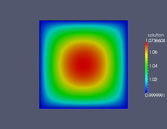
This will execute the Poission solver and give you a rough plot of the solution for 3 seconds. The problem setup is such that we have unit Dirichlet boundary conditions on all boundaries and a unit forcing. You should be able to see this in the plot which is drawn. Here we are using a built-in viewer of PETSc to plot the control points of the solution using:
VecView(x,PETSC_VIEWER_DRAW_WORLD);
where x was our solution vector. This is fine for visual confirmation of correctness in the eyeball norm, but for publications or talks we typically desire higher resolution graphics. For this, we need to output the discretization information and the solution vector and then post-process this. Rerun the example:
./Poisson -save
Running with this option will additionally execute two lines in the code:
IGAWrite(iga,"PoissonGeometry.dat");
IGAWriteVec(iga,x,"PoissonSolution.dat");
These lines dump the needed information into these datafiles.
Python Script
Now, locate the file $PETIGA_DIR/demo/PoissonPlot.py and
examine its contents. We are using a few features of the python
package igakit to read in and parse the discretization
information. First we import the functionality we need:
from igakit.io import PetIGA,VTK
from numpy import linspace
Igakit has a input/ouput module and so we grab the PetIGA and VTK functions from this module. We will also grab a Matlab-like linspace command from numpy. Then we need to read in our data files:
nrb = PetIGA().read("PoissonGeometry.dat")
sol = PetIGA().read_vec("PoissonSolution.dat",nrb)
The first of these reads in the discretization information and
geometry. If no geometry was used, then the control points will be the
Greville abscissa. This gets stored as an igakit NURBS object into the
variable nrb. There is a lot you can do with this object, but
for now we will focus only on writing VTK files. The second line reads
in the solution vector, but requires the NURBS object as well. This is
so we know how to reshape the linear vector array into something that
matches the discretization. Then we can write the VTK file
VTK().write("PoissonVTK.vtk",       # output filename
            nrb,                    # igakit NURBS object
            fields=sol,             # sol is the numpy array to plot
            sampler=uniform,        # specify the function to sample points
            scalars={'solution':0}) # adds a scalar plot to the VTK file
By specifying fields=sol here, we are plotting the solution
vector on top of the geometry contained in the nrb
variable. Associating the solution vector to the plot is not enough to
get the solution plotted in the VTK file. Here, we also specify:
scalars={'solution':0}
where the target of this assignment is a dictionary. Basically a
scalar plot will be created per entry in the dictionary. The string
portion will be what the variable is called in the VTK plot and the
integer portion indicates which component to use of the sol
vector. In this case, we are solving a scalar problem and so there is
only one choice.
The sampler line of this VTK call is not needed. By default, a VTK file will be written, interpolating the solution and geometry at the boundaries of non-zero knot spans. We call these breaks in igakit. However, we can specify a function here to create a finer resolution plot as well. We coded a funtion:
uniform = lambda U: linspace(U[0], U[-1], 100)
where U will be the breaks in the B-spline space in each
dimension. This function simply returns 100 points in between the
first and the last break. This will create a finely interpolated
plot. By executing this python script:
python PoissonPlot.py
you will generate a VTK file called PoissonVTK.vtk. This you
can view with many free viewers such as Paraview or VisIt. Your plot
should look something like the following figure.
Vector Problems
If your problems are vector-valued, then you can output the components
as vector objects in VTK. Compile and execute the
$PETIGA_DIR/demo/NavierStokesKorteweg2D.c code:
make NavierStokesKorteweg2D
./NavierStokesKorteweg2D -nsk_output -ts_max_steps 0
This will run the code with the output option on for zero time steps. We will get a vector out of this code which corresponds to the initial condition. However, this problem has three variables: the first is the density and the last two are the components of the velocity. We can plot these by sightly adjusting our python script:
from igakit.io import PetIGA,VTK
from numpy import linspace
nrb = PetIGA().read("iga.dat")
sol = PetIGA().read_vec("nsk2d0.dat",nrb)
uniform = lambda U: linspace(U[0], U[-1], 100)
VTK().write("nsk0.vtk",
            nrb,
            fields=sol,
            sampler=uniform,
            scalars={'density':0},
            vectors={'velocity':[1,2]})
The main difference is that now we have added a vectors line
along with a list of indices. Intuitively, these components align with
their location in the sol vector as before. Now the resulting
VTK file will contain multiple components for plotting.
Time Dependent Problems
If you let the NavierStokesKorteweg code run for more steps (say
-ts_max_steps 10) then you will get more datafiles of the form
nsk2d*.dat. We can slightly edit our script then to convert
all time steps using the glob module:
from igakit.io import PetIGA,VTK
from numpy import linspace
import glob
nrb = PetIGA().read("iga.dat")
uniform = lambda U: linspace(U[0], U[-1], 100)
for infile in glob.glob("nsk2d*.dat"):
    sol = PetIGA().read_vec(infile,nrb)
    outfile = infile.split(".")[0] + ".vtk"
    VTK().write(outfile,
                nrb,
                fields=sol,
                sampler=uniform,
                scalars={'density':0},
                vectors={'velocity':[1,2]})
The main difference is that we create a list of files to process using
glob and read the solution vector inside of this loop. The output
filename is then created from the input by removing the extension and
adding .vtk.