Creating Geometry with igakit

Objective: At the end of this tutorial you will understand how geometries may be generated with igakit and then be read and used in PetIGA.

Assumptions: I assume that you are familiar with python and have both packages installed and working.

A Brief Overview of igakit

We created igakit to enable both a interface into many low-level routines which are needed to manipulate knot vectors or control point grids as well as a high level interface to simplify the creation of NURBS geometries by hand. These geometries then can be read in to PetIGA for use as a mapping. We also use the package for post-processing solution results from PetIGA. Below we briefly sketch some of the objects available in the package.

• igalib - a python module which contains several submodules. This is a python wrapper around the Fortran module implemented in igalib.f90.
  • bsp - contains interfaces for B-spline related functions such as FindSpan, EvalBasisFunsDers, Greville, InsertKnot, RemoveKnot, DegreeElevate
  • iga - contains interfaces for a few functions that can be used to solve B-spline-based Galerkin problems in python
    • KnotVector - will create a uniform knot vector of user-specified number of elements, polynomial order, inter-element continuity
    • BasisData - returns a series of objects needing to integrate weak form
• nurbs - contains a dimension independent python class (NURBS) which simplifies the usage of routines contained in the igalib module to create and manipulate NURBS curves, surfaces, and volumes.
• io - a module which contains two python classes: PetIGA and VTK which are used to create input/output files suitable to read in by other software.
• cad - a python module which is a collection of python functions which generate commonly used geometries (lines,circles) and perform geometry operations (extrude, join, revolve, ruled, sweep).
• plot - a python module which enables plotting natively in python.

Creating a Geometry

In this tutorial we will not exhaust the possibilities of igakit for generating geometry, but rather explain how igakit geometries can be created and read into PetIGA. We encourage the reader to explore the demo directories of the igakit package for more samples in how igakit can be used to generate NURBS geometries.

As an example, we will create the ever-popular patch test of isogeometric analysis: the quarter annulus. I will write this tutorial as if you are following me in the python interpreter. If you aren’t using ipython, I highly recommend it. First we import the circle functionality from the cad module:

>>> from igakit.cad import circle

Most functions we have implement come with documentation (of various degrees of completeness) built-in to the source code. You can view this by:

>>> help(circle)

where you will see something like the following:

circle(radius=1, center=None, angle=None)
   Construct a NURBS circular arc or full circle

   Parameters
   ----------
   radius : float, optional
   center : array_like, optional
   angle : float or 2-tuple of floats, optional

The third argument of the circle is of interest here. The angle lets us choose a sweep to define our annulus. We can use this to create a circular arc:

>>> from numpy import pi
>>> c1 = circle(angle=(0,pi/2.))

The circle function returns a NURBS object. To get an idea of what you can possibly do with this object, examine the help for it:

>>> help(c1)

You will see a long list of functions and examples of attributes and operations which are possible in the NURBS class. For now, let’s inspect our curve to see what was created. If you are using ipython, you can type:

>>> c1.

and then hit the TAB key. You will see a more concise list of what can be done to this curve:

c1.array      c1.control    c1.evaluate   c1.insert     c1.refine     c1.scale      c1.transform
c1.boundary   c1.copy       c1.extract    c1.knots      c1.remap      c1.shape      c1.translate
c1.breaks     c1.degree     c1.fields     c1.move       c1.remove     c1.slice      c1.transpose
c1.clamp      c1.dim        c1.gradient   c1.plot       c1.reverse    c1.spans      c1.unclamp
c1.clone      c1.elevate    c1.greville   c1.points     c1.rotate     c1.swap       c1.weights

So we see that we can inspect the knot vector:

>>> c1.knots
(array([ 0.,  0.,  0.,  1.,  1.,  1.]),)

As expected, we created a single span of quadratics. The control point grid can also be inspected:

>>> c1.control
array([[  1.00000000e+00,   0.00000000e+00,   0.00000000e+00, 1.00000000e+00],
       [  7.07106781e-01,   7.07106781e-01,   0.00000000e+00, 7.07106781e-01],
       [  2.22044605e-16,   1.00000000e+00,   0.00000000e+00, 1.00000000e+00]])

which are the control points in the 4D space. The first three columns are the x-y-z locations of the control points and the last are the weights. Now we create a second circular arc, this time with a radius of 2:

>>> c2 = circle(radius=2,angle=(0,pi/2.))

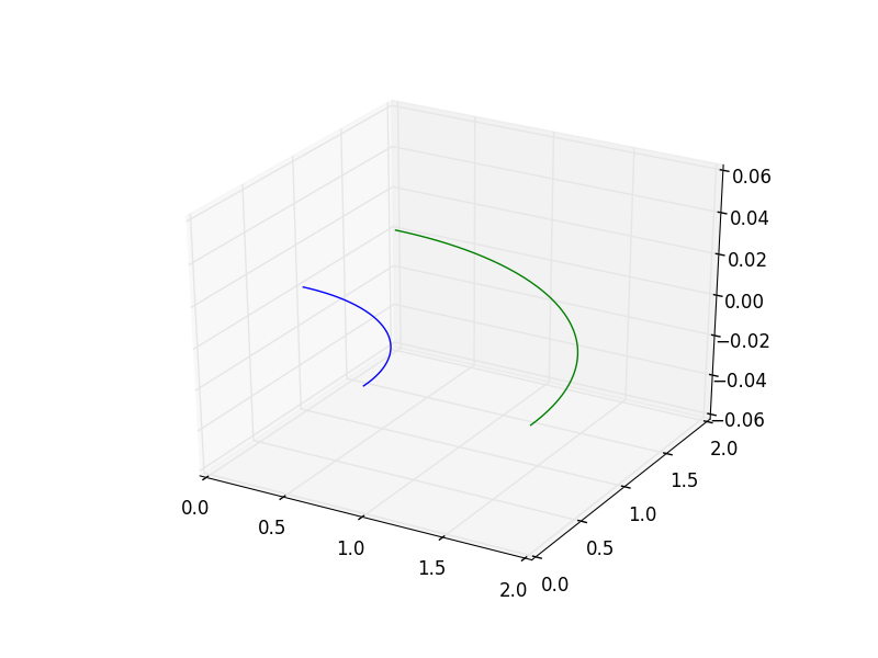
We also have some plotting functionality built into igakit. We will use this now to visually check that our curves have been created as expected:

>>> from igakit.plot import plt
>>> plt.plot(c1,color='b')
>>> plt.plot(c2,color='g')
>>> plt.show()

You will see a 3D window open with the two curves we created that should look something like the following image.

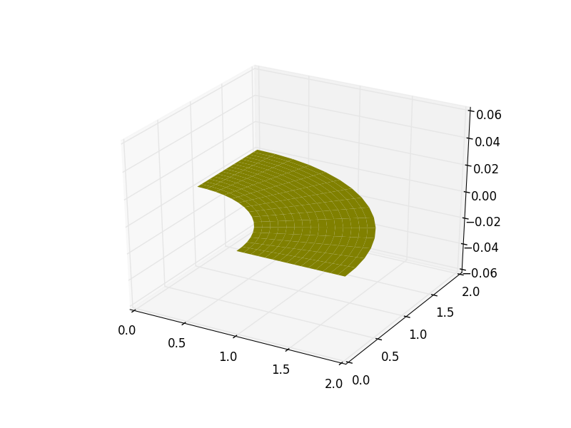
Now, we will create a ruled surface using another function in the cad module, and then also check the result with a plot:

>>> from igakit.cad import ruled
>>> srf = ruled(c1,c2).transpose()
>>> plt.plot(srf)
>>> plt.show()

Reading Geometry Into PetIGA

Now while we have the geometry in hand, we need to prepare it for analysis. Let’s inspect the polynomial orders of the surface that we created:

>>> srf.degree
(1,2)

Here we see that the first direction is the quadratic curve that we had originally, but the ruled operation linearly blended the bounding curves together. Let’s assume that we prefer to use equal polynomial orders in each direction for the annulus. So we need to degree elevate the second direction by one.

>>> srf.elevate(0,1)
>>> srf.degree
(2,2)

We can also inspect the knot vectors:

>>> srf.knots
(array([ 0.,  0.,  0.,  1.,  1.,  1.]), array([ 0.,  0.,  0.,  1.,  1.,  1.]))

Where we see that we have a single nonzero span of bi-quadratics. Since PetIGA does not handle geometry modification internally we need to insert knots here such that the function space matches the one we will use in the analysis portion. To this end, we will create a 10 by 10 element mesh of C1 quadratics by knot insertion:

>>> from numpy import linspace
>>> to_insert = linspace(0,1,11)[1:-1]
>>> srf.refine(0,to_insert)
>>> srf.refine(1,to_insert)
>>> srf.knots
(array([ 0. ,  0. ,  0. ,  0.1,  0.2,  0.3,  0.4,  0.5,  0.6,  0.7,  0.8, 0.9,  1. ,  1. ,  1. ]),
 array([ 0. ,  0. ,  0. ,  0.1,  0.2,  0.3,  0.4,  0.5,  0.6,  0.7,  0.8, 0.9,  1. ,  1. ,  1. ]))

Now the geometry is ready for analysis and to be exported to PetIGA. We use functionality from the io module of igakit.

>>> from igakit.io import PetIGA
>>> PetIGA().write("quarter_annulus.dat",srf)

This will create a datafile that can be read by PetIGA. Now we will use this geometry in the Poisson code with the setup from the previous tutorial, Post-processing Results with igakit. Exit python and compile the demo code $PETIGA_DIR/demo/Poisson.c. I am assuming that the file quarter_annulus.dat that we just created is in this directory. If it is not here, then you will need to move it here. Then run the PetIGA code with these options:

./Poisson -iga_geometry quarter_annulus.dat -iga_view -save

This code solves the Poisson equation with unit Dirichlet boundary conditions everywhere and a unit body force. When we execute this code, we can see what function space was used. Note that this corresponds to what we created in igakit:

IGA: dim=2  dof=1  order=2  geometry=2  rational=1  property=0
Axis 0: periodic=0  degree=2  quadrature=3  processors=1  nodes=12  elements=10
Axis 1: periodic=0  degree=2  quadrature=3  processors=1  nodes=12  elements=10
Partitioning - nodes:    sum=144  min=144  max=144  max/min=1
Partitioning - elements: sum=100  min=100  max=100  max/min=1

Unlike the previous tutorial, the geometry is now flagged as 2D and the rational is flagged to True. If the input geometry is a NURBS then PetIGA detects and compensates for this automatically. Also, if a geometry is used, the basis is mapped automatically with zero code changes required by the user.

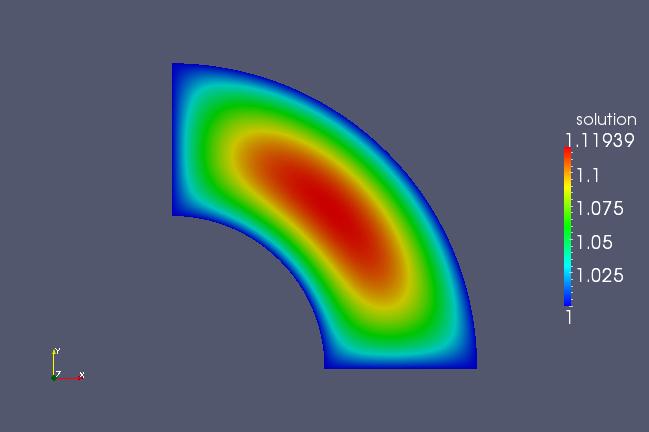
Just as in the previous tutorial, the -save option generates two files (PoissonGeometry.dat and PoissonSolution.dat). Then we can run the same visualization script:

python PoissonPlot.py

which generates PoissonVTK.vtk. However, this time the resulting VTK file encodes the solution on the mapped geometry as in the following image.

Periodicity

Now, what if we did not want to take advantage of the quarter symmetry? How do we generate this geometry? Here I will write a single script which extends the above ideas to all four quadrants:

from igakit import cad
from igakit.io import PetIGA
from numpy import linspace
c1 = cad.circle()
c2 = cad.circle(radius=2)
srf = cad.ruled(c1,c2).transpose().elevate(0,1)
to_insert = linspace(0,0.25,11)[1:-1]
for i in range(4):
    srf.refine(0,i*0.25+to_insert)
    srf.refine(1,i*0.25+to_insert)
PetIGA().write("annulus.dat",srf)

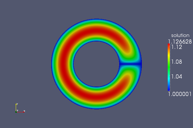
But if run this geometry through the Poisson solver, this geometry will not produce the desired effect, but rather as shown in the following figure.

This is because we set all boundary conditions to one. We need to set the boundaries in the first parametric direction to have periodic boundary conditions. We need to add a line to our script, just before we output the geometry using the PetIGA class:

from igakit import cad
from igakit.io import PetIGA
from numpy import linspace
c1 = cad.circle()
c2 = cad.circle(radius=2)
srf = cad.ruled(c1,c2).transpose().elevate(0,1)
to_insert = linspace(0,0.25,11)[1:-1]
for i in range(4):
    srf.refine(0,i*0.25+to_insert)
    srf.refine(1,i*0.25+to_insert)
srf.unclamp(1) # <----------------------- added this line
PetIGA().write("annulus.dat",srf)

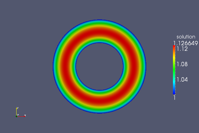
This will modify the geometry to use unclamped knot vectors as opposed to clamped (or open) ones. Now we can rerun the code, specifying the periodicity:

./Poisson -iga_geometry annulus.dat -iga_view -save -iga_periodic 1,0
IGA: dim=2  dof=1  order=2  geometry=2  rational=1  property=0
Axis 0: periodic=1  degree=2  quadrature=3  processors=1  nodes=44  elements=40
Axis 1: periodic=0  degree=2  quadrature=3  processors=1  nodes=39  elements=37
Partitioning - nodes:    sum=1716  min=1716  max=1716  max/min=1
Partitioning - elements: sum=1480  min=1480  max=1480  max/min=1

You will see now that the first direction is flagged periodic and the resulting plot now displays the proper symmetry.